Protein-Level Analysis Tutorial
This tutorial demonstrates a complete protein-level analysis workflow using ProteoPy, from data loading through differential abundance analysis. We use the Karayel et al. (2020) erythropoiesis dataset, which contains protein quantifications across five cell types during red blood cell maturation.
Learning objectives:
Load and annotate proteomics data using the AnnData framework
Perform quality control filtering and visualization
Apply normalization and imputation
Run differential abundance analysis
Visualize and interpret results
Dataset: Karayel, Ö., et al. (2020). Integrative proteomics reveals principles of dynamic phosphosignaling networks in human erythropoiesis. Mol Syst Biol 16, MSB20209813. DOI: 10.15252/msb.20209813
Note: ProteoPy is designed around the AnnData data structure where:
.Xcontains the intensity matrix (samples × proteins).obsstores sample/observation metadata.varstores protein/variable metadata.unsstores unstructured data like color schemes
[1]:
# Jupyter autoreload for development
%load_ext autoreload
%autoreload 2
[2]:
import os
import random
from pathlib import Path
import numpy as np
import pandas as pd
import anndata as ad
import scanpy as sc
import matplotlib.pyplot as plt

import proteopy as pr  # Convention: import proteopy as pr

random.seed(42)

cwd = Path('.').resolve()
root = cwd.parents[1]
os.chdir(root)
/opt/homebrew/Caskroom/miniforge/base/envs/proteopy1/lib/python3.11/site-packages/tqdm/auto.py:21: TqdmWarning: IProgress not found. Please update jupyter and ipywidgets. See https://ipywidgets.readthedocs.io/en/stable/user_install.html
  from .autonotebook import tqdm as notebook_tqdm
Data Loading
ProteoPy provides multiple ways to load data:
pr.read.long()- Load generic long-format tables (sample_id, protein_id, intensity)pr.read.diann()- Load DIA-NN output directlypr.datasets.*- Load built-in example datasets
Here we prepare the Karayel 2020 dataset as TSV files to demonstrate pr.read.long().
[3]:
# Export built-in dataset to TSV files for demonstration
# This creates three files: intensities (long format), sample annotations, and protein annotations
adata = pr.datasets.karayel_2020()

intensities_path = 'data/karayel_2020_intensities.tsv'
sample_annotation_path = 'data/karayel_2020_sample_annotations.tsv'
var_annotation_path = 'data/karayel_2020_protein_annotations.tsv'

# Convert wide matrix to long format (sample_id, protein_id, intensity)
intensities = adata.to_df().reset_index(names='sample_id')
intensities_long = intensities.melt(
    id_vars='sample_id',
    var_name='protein_id',
    value_name='intensity',
    )
intensities_long.to_csv(intensities_path, sep='\t')

adata.obs.to_csv(sample_annotation_path, sep='\t', index=False)
adata.var.to_csv(var_annotation_path, sep='\t', index=False)

del adata
The long-format intensities file contains one row per measurement (sample × protein):
[4]:
!head -n5 {intensities_path}
        sample_id       protein_id      intensity
0       LBaso_rep1      A0A024QZ33;Q9H0G5       15084.2626953125
1       LBaso_rep2      A0A024QZ33;Q9H0G5       15442.2646484375
2       LBaso_rep3      A0A024QZ33;Q9H0G5       13992.021484375
3       LBaso_rep4      A0A024QZ33;Q9H0G5       18426.5390625
[5]:
!head -n5 {sample_annotation_path}
sample_id       cell_type       replicate
LBaso_rep1      LBaso   rep1
LBaso_rep2      LBaso   rep2
LBaso_rep3      LBaso   rep3
LBaso_rep4      LBaso   rep4
[6]:
!head -n5 {var_annotation_path}
protein_id      gene_name
A0A024QZ33;Q9H0G5       NSRP1
A0A024QZB8;A0A0A0MRC7;A0A0D9SFH9;A0A1B0GV71;A0A1B0GW34;A0A1B0GWD3;H3BR00;Q13286;Q13286-2;Q13286-3;Q13286-4;Q13286-5;Q9UBD8      CLN3;CLN3;CLN3;CLN3;CLN3;;CLN3;CLN3;CLN3;CLN3;CLN3;CLN3;CLN3
A0A024R0Y4;O75478       TADA2A
A0A024R216;Q9Y3E1       HDGFRP3;HDGFL3
Loading with pr.read.long()
The long() function reads long-format data into an AnnData object. Key parameters:
level: Specify'protein'or'peptide'level datasample_annotation: Optional metadata for samples (→.obs)var_annotation: Optional metadata for proteins/peptides (→.var)fill_na: Value to fill missing intensities (e.g.,0for missing values)
[7]:
adata = pr.read.long(
    intensities=intensities_path,
    level='protein',
    sample_annotation=sample_annotation_path,
    var_annotation=var_annotation_path,
    fill_na=0,
)

adata
[7]:
AnnData object with n_obs × n_vars = 20 × 7758
    obs: 'sample_id', 'cell_type', 'replicate'
    var: 'protein_id', 'gene_name'
[8]:
# Validate that the loaded data conforms to proteodata format
from proteopy.utils.anndata import check_proteodata

check_proteodata(adata)
[8]:
(True, 'protein')
Alternative: Annotating Data After Loading
If you load data without annotations, you can add them later using the pr.ann module:
# Add sample annotations from a DataFrame
pr.ann.obs(adata, df=sample_df, obs_on='sample_id', df_on='sample_id')
pr.ann.samples(...)  # Alias for pr.ann.obs

# Add protein/peptide annotations
pr.ann.var(adata, df=protein_df, var_on='protein_id', df_on='protein_id')
These functions merge annotation DataFrames into .obs or .var by matching on key columns.
Storing Metadata in .uns
The .uns slot stores unstructured data like color schemes and analysis parameters. ProteoPy plotting functions can read color mappings from .uns['colors_<category>']:
[9]:
# Store color scheme in .uns for consistent plotting across the tutorial
adata.uns['colors_cell_type'] = {
    "LBaso": "#D91C5C",
    "Ortho": "#F6922F",
    "Poly": "#262261",
    "ProE&EBaso": "#1B75BB",
    "Progenitor": "#D6DE3B",
}

# Define haemoglobin proteins for highlighting (marker proteins in erythropoiesis)
haemoglobin = {
    'F8W6P5': 'HBB1',
    'P69905': 'HBA1',
    'P02100': 'HBE1',
    'A0A2R8Y7X9;P69891': 'HBG1',
}

# Store differentiation order once for consistent plotting
adata.uns['diff_order'] = ['Progenitor', 'ProE&EBaso', 'LBaso', 'Poly', 'Ortho']
Handling Missing Values and Zeros
In bottom-up proteomics, missing values are pervasive and arise from two fundamentally different mechanisms:
Missing Not At Random (MNAR): The protein abundance falls below the instrument’s detection limit. Because the signal is absent due to low abundance, this is a systematic, non-random gap. In practice, MNAR values can be treated as true zeros — the protein was not detected and its abundance is at or near zero.
Missing At Random (MAR): The protein is present at detectable levels but was not measured due to stochastic effects in data acquisition (e.g., under-sampling in data-dependent acquisition). These are genuinely missing observations (NA/NaN) — the value exists but is unknown.
How ProteoPy treats zeros and NAs:
ProteoPy distinguishes between 0 and np.nan in the data matrix (.X):
Zeros are treated as a real quantity in algorithms — they represent proteins that were not detected or fell below the detection limit. Functions such as mean, median, normalization, and statistical tests include zeros in their calculations.
NAs (``np.nan``) are not taken into account. Most functions either skip them (e.g., using
np.nanmean) or raise an error when NAs are present (e.g.,pr.tl.differential_abundance()requires imputed or complete data).
Because different workflows require different handling, ProteoPy does not automatically convert between zeros and NAs. Instead, this is left to the user via function-level parameters:
Parameter |
Description |
|---|---|
|
Temporarily treat zeros as missing values for this operation |
|
Replace NAs with a specified value (e.g., |
Example: The same data can yield different results depending on how zeros are handled:
import numpy as np

# Sample data: 3 samples, 1 protein with a zero value
# adata.X = [[100], [0], [200]]

# Counting "detected" proteins per sample:
pr.pl.n_proteins_per_sample(adata, zero_to_na=False)  # Returns [1, 1, 1] — zero counts as detected
pr.pl.n_proteins_per_sample(adata, zero_to_na=True)   # Returns [1, 0, 1] — zero treated as missing

# Filtering by completeness:
pr.pp.filter_var_completeness(adata, min_fraction=1.0, zero_to_na=False)  # Keeps protein (100% "complete")
pr.pp.filter_var_completeness(adata, min_fraction=1.0, zero_to_na=True)   # Removes protein (only 67% complete)
In this tutorial, we load the data with fill_na=0, meaning all undetected proteins, regardless of their source of missingness, start represented as zeros. We then use zero_to_na=True at the function level in QC and filtering steps so that zeros are treated as missing, and later convert zeros to np.nan explicitly before log transformation and imputation.
Quality Control and Data Filtering
Quality control in proteomics involves:
Visualizing data characteristics (abundance distributions, completeness)
Removing contaminants (e.g., common laboratory contaminants)
Filtering samples/proteins with insufficient measurements
Protein Abundance Rank Plot
The abundance rank plot shows median protein intensities across samples, useful for identifying highly abundant proteins and potential contaminants:
[10]:
# Haemoglobin proteins are highlighted
pr.pl.abundance_rank(
    adata,
    color='cell_type',
    log_transform=10,
    zero_to_na=True,            # Treat zeros as missing values
    color_scheme=adata.uns["colors_cell_type"],
    summary_method='median',
    highlight_vars=list(haemoglobin.keys()),
    var_labels_key='gene_name', # Use gene names instead of protein IDs for labels
    )
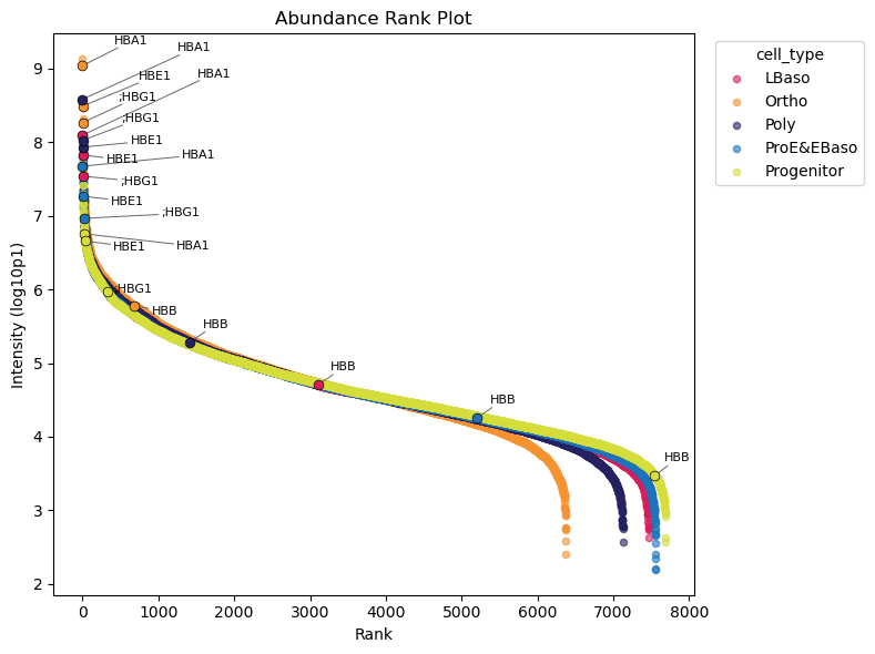
📊 Higher abundance of haemoglobin proteins in the protein distribution is expected and they are expected to increase during erythropoiesis. The abundance rank plot confirms this with exception of HBB proteins.
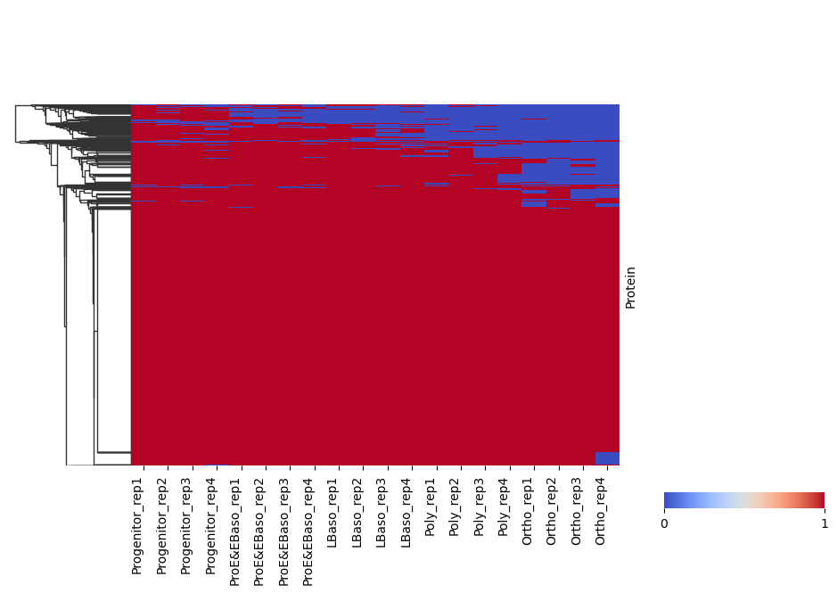
Binary Detection Heatmap
pr.pl.binary_heatmap() converts intensities into a binary matrix (present/absent) and visualizes it as a heatmap. This is useful for quickly checking detection patterns across samples and proteins.
Here, we consider proteins with log2 intensity > 0 as present and order samples by differentiation stage.
[11]:
# Binary heatmap: proteins above threshold are encoded as 1 (present), otherwise 0
pr.pl.binary_heatmap(
adata,
threshold=0,
fill_na=0,
order_by='cell_type',
order=adata.uns['diff_order'],
col_cluster=False,
row_cluster=True,
figsize=(10, 6),
)
/opt/homebrew/Caskroom/miniforge/base/envs/proteopy1/lib/python3.11/site-packages/seaborn/matrix.py:560: UserWarning: Clustering large matrix with scipy. Installing `fastcluster` may give better performance.
  warnings.warn(msg)
Removing Contaminants
Common contaminants (keratins, BSA, trypsin, etc.) should be removed. ProteoPy can download contaminant databases and filter them out:
[12]:
# Download contaminant FASTA (sources: 'frankenfield2022', 'gpm-crap')
contaminants_path = pr.download.contaminants(source='frankenfield2022')

# Remove proteins matching contaminant sequences
pr.pp.remove_contaminants(
    adata,
    contaminant_path=contaminants_path,
    inplace=True,  # Modify adata directly (default behavior)
    )
Removed 12 contaminating proteins.
/Users/leventetn/Documents/Proteopy/proteopy/proteopy/download/contaminants.py:140: UserWarning: File already exists at data/contaminants_frankenfield2022_2026-02-28.fasta. Use force=True to overwrite.
  warnings.warn(
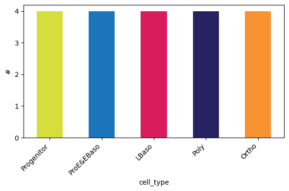
Sample Distribution
Check how many samples (replicates) exist per experimental group:
[13]:
pr.pl.n_samples_per_category(
        adata,
        category_key='cell_type',
        color_scheme=adata.uns['colors_cell_type'],
        order=adata.uns['diff_order'],
        )
Filtering Functions
ProteoPy provides filtering at both sample (obs) and protein/peptide (var) levels:
Variable-level filtering (``pr.pp.filter_var*``):
filter_var()- General filtering per variable by any criteriafilter_var_completeness()- Filter by fraction/count of non-missing valuesfilter_proteins_by_peptide_count()- Filter proteins by number of peptides (peptide-level data)
Sample-level filtering (``pr.pp.filter_samples*``):
filter_samples()- General filtering per sample by any criteria.filter_samples_completeness()- Filter by minimum protein count or minimum fraction of non-missing proteinsfilter_samples_by_category_count()- Ensure minimum samples per metadata categroy/group
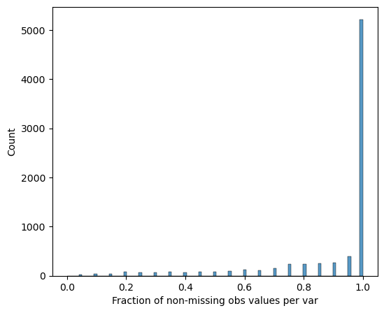
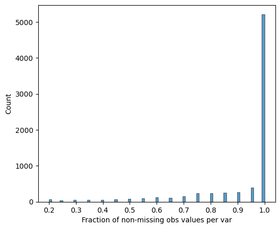
[14]:
# Visualize protein completeness before filtering
pr.pl.completeness_per_var(adata, zero_to_na=True)
[15]:
# Require 100% completeness within at least one cell type (group_by='cell_type')
# This keeps proteins that are consistently measured in at least one cell type.
pr.pp.filter_var_completeness(
    adata,
    min_fraction=1,
    group_by='cell_type',
    zero_to_na=True,
    )
277 var removed
[16]:
# Verify completeness after filtering
pr.pl.completeness_per_var(adata, zero_to_na=True)
Sample Quality Assessment
Examine the number of detected proteins per sample. The order_by and order parameters control how samples are arranged:
[17]:
# Per-sample protein counts (individual bars)
pr.pl.n_proteins_per_sample(
    adata,
    zero_to_na=True,
    order_by='cell_type',
    order=adata.uns['diff_order'],
    color_scheme=adata.uns['colors_cell_type'],
    xlabel_rotation=45,
    )
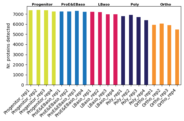
📊 We observe a trend of decreasing detected protein count along differentiation trajectory
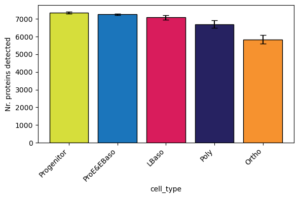
[18]:
# Grouped by cell type (boxplot per group) - reproduces Figure 1C from Karayel et al.
pr.pl.n_proteins_per_sample(
    adata,
    zero_to_na=True,
    group_by='cell_type',  # Aggregate samples into boxplots per group
    order=adata.uns['diff_order'],
    color_scheme=adata.uns['colors_cell_type'],
    xlabel_rotation=45,
    )
[19]:
# Remove samples with fewer than 6000 detected proteins
pr.pp.filter_samples(adata, min_count=6000)
0 obs removed
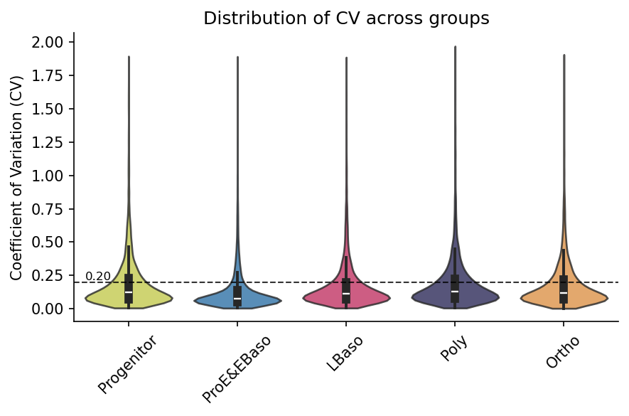
Coefficient of Variation (CV)
The CV measures variability within pre-defined sample groups. When grouping by cell type, variation comes from the replicate samples so the CV represents technical variability. Lower CV indicates better reproducibility:
[20]:
# Calculate CV per protein within each cell type (stored in adata.var)
pr.pp.calculate_cv(adata, group_by='cell_type', min_samples=3)
[21]:
# Visualize CV distribution per group (hline shows typical 20% CV threshold)
pr.pl.cv_by_group(
    adata,
    group_by='cell_type',
    color_scheme=adata.uns["colors_cell_type"],
    figsize=(6, 4),
    xlabel_rotation=45,
    order=adata.uns['diff_order'],
    hline=0.2,  # Reference line at 20% CV
    )
Using existing CV data from adata.varm['cv_by_cell_type_X'].
Data Transformations
Proteomics data typically requires:
Log transformation - Reduces skewness from normal distribution, stabilizes the mean–variance relationship and makes fold changes symmetric
Normalization - Corrects for systematic technical variation between samples
Imputation - Handles missing values for downstream statistical analysis
Log Transformation
[22]:
# Convert zeros to NaN (missing values) and log2 transform
# Note: Save raw data in `layers` and then modigy adata.X directly
adata.layers['raw'] = adata.X.copy()
adata.X[adata.X == 0] = np.nan
adata.X = np.log2(adata.X)
Normalization
Options:
median normalization
[23]:
# Visualize intensity distributions between samples first
pr.pl.intensity_box_per_sample(
    adata,
    order_by='cell_type',
    order=adata.uns['diff_order'],
    zero_to_na=True,
    color_scheme=adata.uns['colors_cell_type'],
    xlabel_rotation=45,
    figsize=(9, 6),
    )
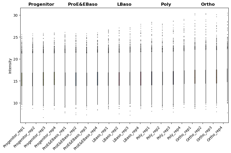
[23]:
<Axes: ylabel='Intensity'>
[24]:
# Apply median normalization (method='median_ref' uses a reference sample)
pr.pp.normalize_median(
    adata,
    method='median_ref',
    log_space=True, # log_space=True indicates data is already log-transformed
    )
[25]:
# After normalization: distributions should be aligned
pr.pl.intensity_box_per_sample(
    adata,
    order_by='cell_type',
    order=adata.uns['diff_order'],
    zero_to_na=True,
    color_scheme=adata.uns['colors_cell_type'],
    xlabel_rotation=45,
    figsize=(9, 6),
    )
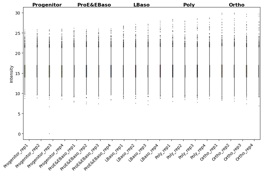
[25]:
<Axes: ylabel='Intensity'>
Imputation
As discussed above, often missing values in proteomics are MNAR — proteins below the detection limit. Down-shift imputation addresses this by sampling replacement values from a distribution shifted below the observed measurements, assuming that missing proteins have low but non-zero abundance:
[26]:
# Impute missing values using down-shift method
# downshift: How many std devs below mean to center imputed values
# width: Width of the imputation distribution (std devs)
pr.pp.impute_downshift(
    adata,
    downshift=1.8,
    width=0.3,
    zero_to_nan=True,
    random_state=123,  # For reproducibility
    )
[27]:
# Nr of measured and imputed values
mask = np.asarray(adata.layers["imputation_mask_X"], dtype=bool)
measured_n = int((~mask).sum())
imputed_n = int(mask.sum())
print(f"Measured: {measured_n:,} values ({100*measured_n/(measured_n+imputed_n):.1f}%)")
print(f"Imputed: {imputed_n:,} values ({100*imputed_n/(measured_n+imputed_n):.1f}%)")
Measured: 136,962 values (91.7%)
Imputed: 12,418 values (8.3%)
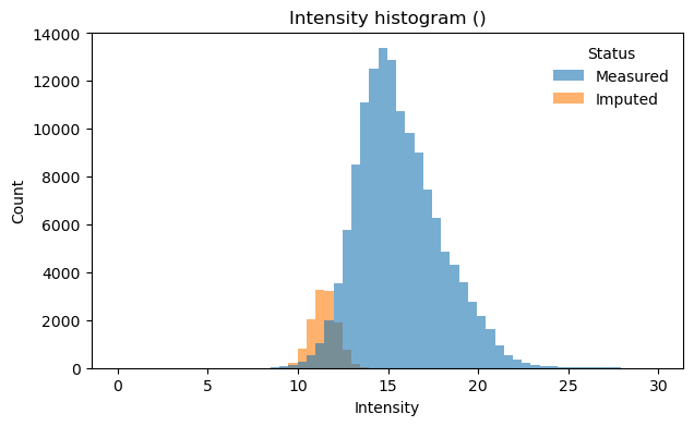
[28]:
# Visualize intensity distribution with imputed values highlighted
# Combined histogram across all samples
pr.pl.intensity_hist(
adata,
color_imputed=True, # Color imputed vs measured values differently
density=False,
)
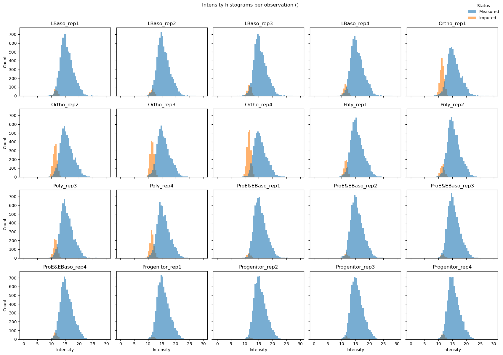
# Per-sample histograms (small multiples)
pr.pl.intensity_hist(
adata,
color_imputed=True,
per_obs=True, # One subplot per sample
ncols=5,
legend_loc="upper right",
density=False,
figsize=(17, 12),
)
Dimensionality Reduction and Sample Clustering
ProteoPy integrates with scanpy for dimensionality reduction. PCA and UMAP reveal sample relationships and confirm expected biological groupings.
[29]:
# PCA using scanpy (ProteoPy AnnData is fully compatible)
sc.tl.pca(adata)
sc.pl.pca_variance_ratio(adata, n_pcs=50, log=True)
sc.pl.pca(
    adata,
    color='cell_type',
    dimensions=(0, 1),
    ncols=2,
    size=90,
    palette=adata.uns['colors_cell_type'],
    )
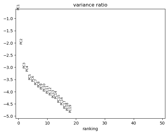
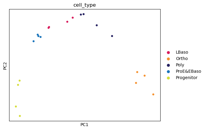
📊 The first two principal components resolve the differentiation trajectory indicating that the highest source of variation is the biological process of erythropoiesis.
[30]:
# UMAP for non-linear dimensionality reduction
sc.pp.neighbors(adata, n_neighbors=6)
sc.tl.umap(adata)
sc.pl.umap(
    adata,
    color='cell_type',
    size=100,
    palette=adata.uns['colors_cell_type'],
    )
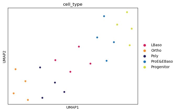
📊 Dimensionality reduction identifies cell type clusters.
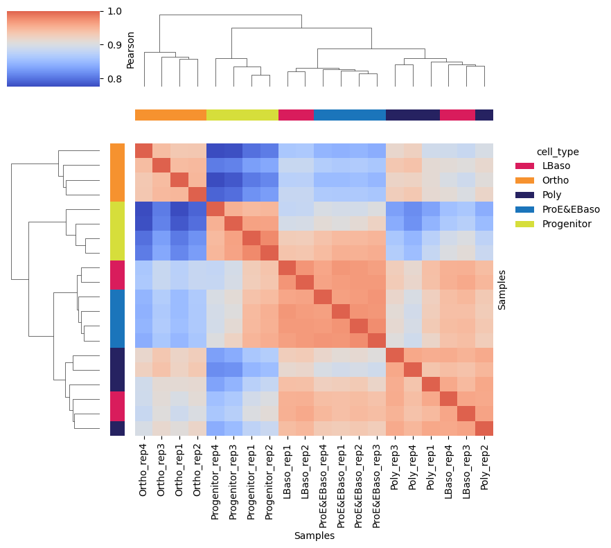
Sample Correlation Matrix
A hierarchically clustered correlation matrix shows sample similarity:
[31]:
# Clustered sample correlation heatmap with cell type annotation on margins
pr.pl.sample_correlation_matrix(
    adata,
    method="pearson",
    margin_color="cell_type",  # Color bar annotation
    color_scheme=adata.uns["colors_cell_type"],
    xticklabels=True,
    figsize=(9, 8),
    linkage_method='average',
    )
Highly Variable Proteins
Identifying highly variable proteins (HVPs) highlights proteins that vary most across samples - these often drive biological differences between conditions:
[32]:
# Use scanpy's HVG detection (marks top 250 most variable proteins in adata.var)
sc.pp.highly_variable_genes(
    adata,
    n_top_genes=250,
    inplace=True,
    )
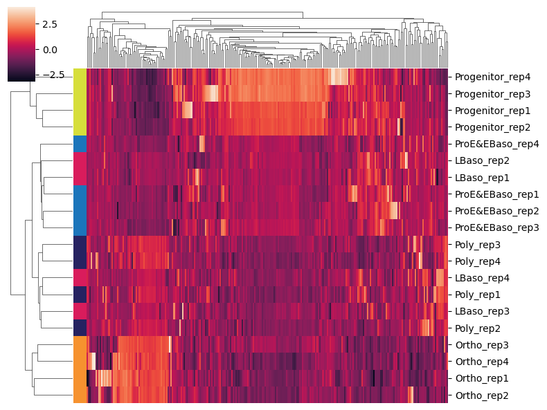
[33]:
# Subset to highly variable proteins and plot clustered heatmap
adata_hvg = adata[:, adata.var['highly_variable']].copy()

sc.pl.clustermap(
    adata_hvg,
    obs_keys='cell_type',
    z_score=1,          # Z-score normalize per protein (row)
    figsize=(8, 6),
    dendrogram_ratio=0.15,
    show=True,
    xticklabels=False,  # Too many proteins for labels
    )
Differential Abundance Analysis
ProteoPy performs statistical testing to identify proteins that differ significantly between conditions.
Running Statistical Tests
Available methods:
ttest_two_sample- Two-sample t-test (assumes equal variance)welch- Welch’s t-test (unequal variance)
Test modes:
one_vs_rest: Compare each group to all others combined (default when
setup={})pairwise: Specify explicit comparisons with
setup={'group1': 'A', 'group2': 'B'}
[34]:
# One-vs-rest t-tests for each cell type (results stored in adata.varm)
pr.tl.differential_abundance(
    adata,
    method="ttest_two_sample",
    group_by='cell_type',
    setup={},               # Empty = one-vs-rest for all groups
    multitest_correction='bh',  # Benjamini-Hochberg FDR correction
    alpha=0.05,
    space='log',            # Data is in log space
    )
Saved test results in .varm['ttest_two_sample;cell_type;LBaso_vs_rest']
Saved test results in .varm['ttest_two_sample;cell_type;Ortho_vs_rest']
Saved test results in .varm['ttest_two_sample;cell_type;Progenitor_vs_rest']
Saved test results in .varm['ttest_two_sample;cell_type;ProE_EBaso_vs_rest']
Saved test results in .varm['ttest_two_sample;cell_type;Poly_vs_rest']
Accessing Test Results
Test results are stored in adata.varm slots. Use pr.get.tests() to see available results:
[35]:
# List all stored test results
pr.get.tests(adata)
[35]:
| key | key_group | test_type | group_by | design | design_label | design_mode | layer | |
|---|---|---|---|---|---|---|---|---|
| 0 | ttest_two_sample;cell_type;LBaso_vs_rest | ttest_two_sample;cell_type;one_vs_rest | ttest_two_sample | cell_type | LBaso_vs_rest | LBaso vs rest | one_vs_rest | None |
| 1 | ttest_two_sample;cell_type;Ortho_vs_rest | ttest_two_sample;cell_type;one_vs_rest | ttest_two_sample | cell_type | Ortho_vs_rest | Ortho vs rest | one_vs_rest | None |
| 2 | ttest_two_sample;cell_type;Progenitor_vs_rest | ttest_two_sample;cell_type;one_vs_rest | ttest_two_sample | cell_type | Progenitor_vs_rest | Progenitor vs rest | one_vs_rest | None |
| 3 | ttest_two_sample;cell_type;ProE_EBaso_vs_rest | ttest_two_sample;cell_type;one_vs_rest | ttest_two_sample | cell_type | ProE_EBaso_vs_rest | ProE EBaso vs rest | one_vs_rest | None |
| 4 | ttest_two_sample;cell_type;Poly_vs_rest | ttest_two_sample;cell_type;one_vs_rest | ttest_two_sample | cell_type | Poly_vs_rest | Poly vs rest | one_vs_rest | None |
Use pr.get.differential_abundance_df() to retrieve results as a DataFrame with filtering:
[36]:
# Get significant proteins across all one-vs-rest tests (|logFC| >= 1, p_adj < 0.05)
pr.get.differential_abundance_df(
    adata,
    key_group='ttest_two_sample;cell_type;one_vs_rest',  # All one-vs-rest tests
    min_logfc=1,        # Minimum absolute log2 fold change
    max_pval=0.05,      # Maximum adjusted p-value
    sort_by='pval_adj', # Sort by adjusted p-value
    )
[36]:
| var_id | test_type | group_by | design | mean1 | mean2 | logfc | tstat | pval | pval_adj | is_diff_abundant | |
|---|---|---|---|---|---|---|---|---|---|---|---|
| 0 | Q8IXW5;Q8IXW5-2 | ttest_two_sample | cell_type | Ortho_vs_rest | 21.060375 | 12.935327 | 8.125048 | 23.517326 | 5.778442e-15 | 3.114776e-11 | True |
| 1 | E7ESC6 | ttest_two_sample | cell_type | Ortho_vs_rest | 19.692222 | 16.984114 | 2.708108 | 16.811764 | 1.885384e-12 | 7.040966e-10 | True |
| 2 | Q8TB52 | ttest_two_sample | cell_type | Ortho_vs_rest | 16.234364 | 13.902348 | 2.332016 | 15.007092 | 1.278869e-11 | 2.449197e-09 | True |
| 3 | Q7Z333;Q7Z333-4 | ttest_two_sample | cell_type | Ortho_vs_rest | 16.963578 | 15.899757 | 1.063821 | 14.861999 | 1.504470e-11 | 2.613229e-09 | True |
| 4 | O43516;O43516-2;O43516-3;O43516-4 | ttest_two_sample | cell_type | Progenitor_vs_rest | 15.411008 | 11.522910 | 3.888098 | 16.436716 | 2.763870e-12 | 1.104769e-08 | True |
| ... | ... | ... | ... | ... | ... | ... | ... | ... | ... | ... | ... |
| 956 | Q6UW63 | ttest_two_sample | cell_type | Progenitor_vs_rest | 15.015388 | 13.067117 | 1.948270 | 2.778024 | 1.240691e-02 | 4.915014e-02 | True |
| 957 | Q9UPY3 | ttest_two_sample | cell_type | Progenitor_vs_rest | 13.912874 | 12.656495 | 1.256379 | 2.777509 | 1.242059e-02 | 4.916237e-02 | True |
| 958 | J9JIC5;Q9HAS0 | ttest_two_sample | cell_type | Progenitor_vs_rest | 13.641169 | 12.517267 | 1.123901 | 2.774577 | 1.249870e-02 | 4.931474e-02 | True |
| 959 | H0YH69;Q9HBU6 | ttest_two_sample | cell_type | Progenitor_vs_rest | 13.984629 | 12.503137 | 1.481492 | 2.771020 | 1.259412e-02 | 4.953421e-02 | True |
| 960 | A0A075B6E4;A0A0A6YYI5;G5E9M7;G5E9M9;Q14135;Q14... | ttest_two_sample | cell_type | Progenitor_vs_rest | 12.950283 | 11.872185 | 1.078098 | 2.766072 | 1.272799e-02 | 4.990309e-02 | True |
961 rows × 11 columns
Visualization
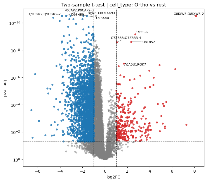
Volcano Plot
Volcano plots show the relationship between fold change (x) and statistical significance (y):
[37]:
# Volcano plot for Ortho vs rest comparison
pr.pl.volcano_plot(
    adata,
    varm_slot='ttest_two_sample;cell_type;Ortho_vs_rest',
    fc_thresh=1,        # Fold change threshold lines
    pval_thresh=0.05,   # P-value threshold line
    xlabel='log2FC',
    ylabel_logscale=True,
    top_labels=5,       # Label top 5 most significant
    figsize=(8, 7),
    )
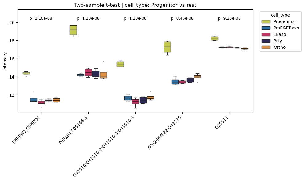
Box Plots of Top Differentially Abundant Proteins
Examine individual protein intensity distributions:
[38]:
# Box plots for top 5 differentially abundant proteins (Progenitor vs rest)
pr.pl.differential_abundance_box(
    adata,
    varm_slot='ttest_two_sample;cell_type;Progenitor_vs_rest',
    top_n=5,
    color_scheme=adata.uns['colors_cell_type'],
    order=adata.uns['diff_order'],
    )
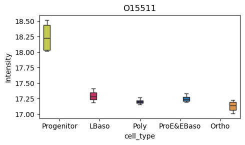
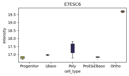
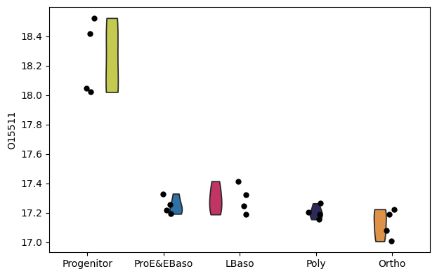
[39]:
# Box plot for a specific protein of interest
pr.pl.box(
    adata,
    keys=['O15511', 'E7ESC6'],
    group_by='cell_type',
    order=['Progenitor', 'LBaso', 'Poly', 'ProE&EBaso', 'Ortho'],
    color_scheme=adata.uns['colors_cell_type'],
    figsize=(5,3),
    )
[40]:
# Alternative: use scanpy's violin plot
sc.pl.violin(
    adata,
    keys=['O15511'],
    groupby='cell_type',
    order=adata.uns['diff_order'],
    size=6,
    xlabel=None,
    )
Hierarchical Clustering of Proteins
ProteoPy provides tools for clustering proteins by their expression profiles across conditions. This is useful for identifying co-regulated protein groups.
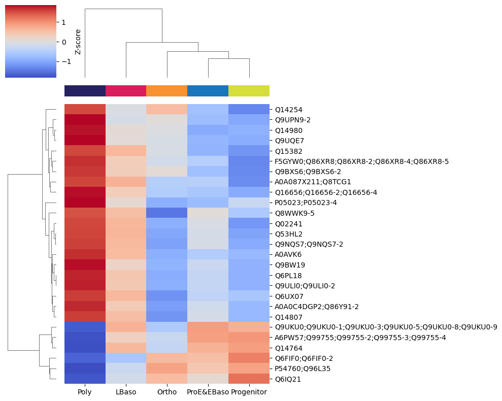
Profile Heatmap
First, visualize the expression profiles of differentially abundant proteins:
[41]:
# Get differentially abundant proteins for Poly vs rest
df = pr.get.differential_abundance_df(
    adata,
    keys='ttest_two_sample;cell_type;Poly_vs_rest',
    )
diff_prots = df[df['pval_adj'] <= 0.05]

# Heatmap of mean intensities per cell type for these proteins
pr.pl.hclustv_profiles_heatmap(
    adata,
    group_by='cell_type',
    selected_vars=diff_prots['var_id'],
    yticklabels=True,
    margin_color=True,
    color_scheme=adata.uns['colors_cell_type'],
    )
Building the Hierarchical Clustering Tree
pr.tl.hclustv_tree() builds a hierarchical clustering dendrogram based on mean expression profiles:
[42]:
# Build hierarchical clustering tree (stored in adata.uns)
pr.tl.hclustv_tree(
    adata,
    group_by='cell_type',
    selected_vars=diff_prots['var_id'],
    verbose=False,
    )
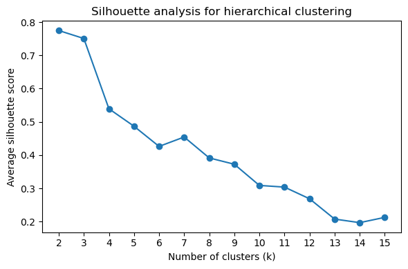
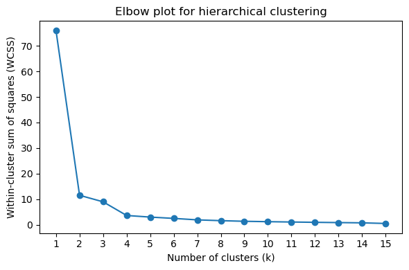
Determining Optimal Cluster Number
Use silhouette scores and elbow plots to determine the optimal number of clusters (k):
[43]:
# Silhouette score plot (higher = better cluster separation)
pr.pl.hclustv_silhouette(adata, verbose=False)
[44]:
# Elbow plot (look for the "elbow" where inertia decrease slows)
pr.pl.hclustv_elbow(adata, verbose=False)
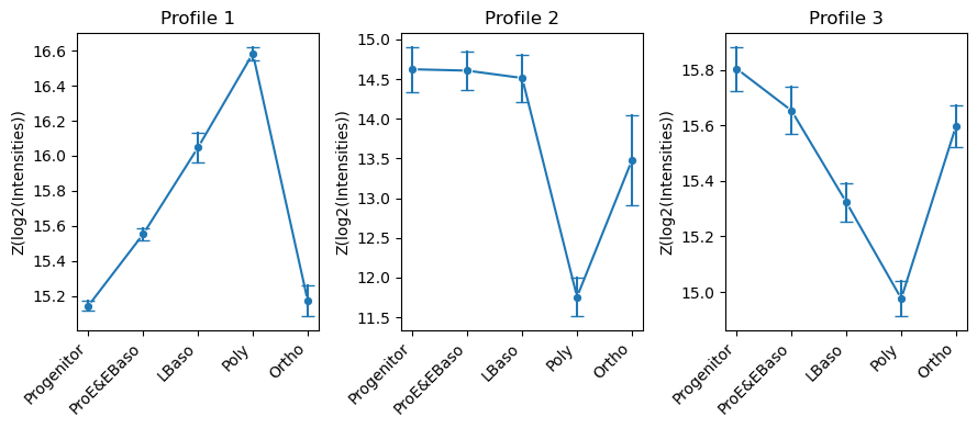
Cluster Assignment and Profile Visualization
Cut the dendrogram at k clusters and compute mean profiles per cluster:
[45]:
# Assign proteins to k=3 clusters and compute cluster profiles
pr.tl.hclustv_cluster_ann(adata, k=3, verbose=False)
pr.tl.hclustv_profiles(adata, verbose=False)
[46]:
# Visualize cluster profiles: mean ± std intensity across cell types for each cluster
pr.pl.hclustv_profile_intensities(
    adata,
    group_by='cell_type',
    order=adata.uns['diff_order'],
    ylabel='Z(log2(Intensities))',
    verbose=False,
    n_cols=3,
    figsize=(9, 4),
    )
Summary
This tutorial covered the core ProteoPy workflow for protein-level analysis:
Data loading -
pr.read.long()for generic formats,pr.read.diann()for DIA-NN outputAnnotation -
pr.ann.obs()andpr.ann.var()for adding metadataQuality control -
pr.pp.filter_*()for filtering,pr.pl.*for visualizationTransformation - Log transformation,
pr.pp.normalize_median(),pr.pp.impute_downshift()Statistical analysis -
pr.tl.differential_abundance()withpr.get.differential_abundance_df()Clustering -
pr.tl.hclustv_*()for hierarchical clustering of expression profiles
ProteoPy integrates seamlessly with scanpy for dimensionality reduction (PCA, UMAP) and other single-cell analysis tools.
For more information, see the ProteoPy documentation.